Neural Network precision pitfalls in the wild
In my work, I draw on concepts from computational geometry and graphics, often demanding high-precision guarantees. A typical case is sampling an object’s implicit function to generate a parameterised form for downstream use.
Neural networks tend to be a perfect fit for such problems. They are great at expressing complex, nonlinear structures, are differentiable, and can be infinitely precise. In theory, the precision part is well-supported, but in practice, let’s explore the challenges that arise. I’ll take a top-bottom approach, grounding the problem scenarios in the real-world, and then get into pitfalls to lookout for and even establish certain error bounds.
Problem setting
To reflect on an actual use-case (from my work), let \(F\colon\mathbb{R}^3\to\Delta^1\subset\mathbb{R}^2\) be our neural network. For illustration we restrict to a one‐dimensional slice in \(\mathbb{R}^3\). Fix two coordinates \(x_2^*,x_3^*\) and let
\[L \;=\;\bigl\{(t,x_2^*,x_3^*) : t\in[t_{\min},\,t_{\max}]\bigr\}\]for some suitably chosen interval \([t_{\min},t_{\max}]\). \(F\) is trained by sampling the two ground-truth curves shown in the plot below.
\[p_0(t) \quad\text{and}\quad p_1(t)\;=\;1 - p_0(t)\]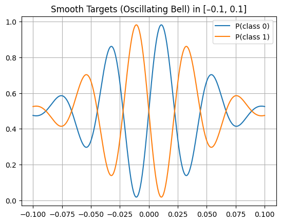
Figure 1. Plot of \(p_0(x)=0.5+0.5\sin(45\pi x)e^{-300x^2}\) and its complement \(1 - p_0(x)\).
We shall use JAX/FLAX for all experiments in this work.
Pitfalls
Now, given we have a well trained Neural Network \(F\) that approximates a function. How reliably can we sample \(F\)?
Error accumulation in a forward pass
A network can fit such data very easily, given decent complexity in it’s architecture. However, there is also an unintended effect on the stability of its predictions as the numbers flow through a forward pass. Let’s analyse this through a gridsearch over the depth and width of a simple ResNet.
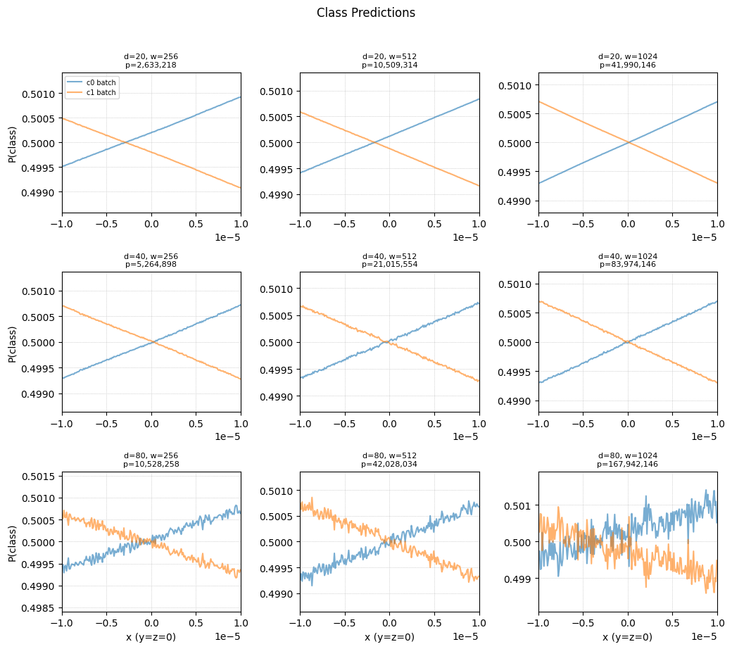
Figure 2. Grid search for accumulated error over depth and width of network. Default matmul settings used here.
In the above image we sample a neural network in a small interval, where the two classes overlap. For many geometry applications this is an area of interest, since it contains a zero for \(F_1-F_0\). However, because of noise accumulated, there exist multiple zeroes here.
This raises a fair few questions!
- Why does this noise occur?
- Why is it exaggerated for bigger networks?
- Given a network, can we find bounds for it?
These questions force us to quantify, how errors can be injected in a forward pass. Some of the relevant pieces being:
\[u \;=\; 2^{-23}\;\approx1.19\times10^{-7}, \qquad \gamma_n \;=\;\frac{n\,u}{1 - n\,u}\;\approx\;n\,u.\]Here \(u\) is the unit round-off for IEEE-754 float32 (not what is used by default!), and \(\gamma_n\) is the worst-case relative error of an \(n\)-term dot product.
Note: In most famous Deep Learning libraries, the default matmul settings use a mix of float32 and TF32 calculations depending on the kernel employed. This increases the instability! More on this later.
| Component | Fan-in / ops | Worst-case relative error bound | Notes / mitigation |
|---|---|---|---|
| Dense layer | \(n\) multiplies + adds | \(\le\gamma_n\) | narrower layers ⇒ smaller \(\gamma_n\) |
| ReLU / skip-add | 1 compare + 1 add | \(\le u < \gamma_1\) | negligible |
| BatchNorm / LayerNorm | ≈3 ops | \(\le3\,u < \gamma_3\) | normalises activations ⇒ later \(\gamma\) shrink |
| TF32 matmul (default of most libraries) | same count, 10-bit mantissa | \(\gamma_n^{\rm TF32}\approx n\,2^{-10}\) | Can be made more precise, pushing the error down |
Because each layer \(\ell\) injects at most a \(\gamma_{n_\ell}\) relative slip, chaining \(L\) layers gives (dropping \(O(u^2)\) terms):
\[\hat f(x) = f(x)\,\prod_{\ell=1}^L(1+\delta^{(\ell)}) \;=\; f(x)\,\bigl(1 + \underbrace{\sum_{\ell=1}^L\delta^{(\ell)}}_{\displaystyle\varepsilon_{\rm acc}(x)}\bigr), \quad \bigl|\delta^{(\ell)}\bigr|\le\gamma_{n_\ell} \;\Longrightarrow\; \bigl|\varepsilon_{\rm acc}(x)\bigr|\le\sum_{\ell=1}^L\gamma_{n_\ell}.\]That is, the total forward-pass error is bounded by the sum of each layer’s \(\gamma\). See Appendix for the detailed proof.
Kernel Drift for different batch sizes
When you compare “single-input” (loop) inference to “multi-input” (batch) inference, you’re driving two different reduction pipelines, meaning they can produce slightly different sums in floating-point. Hence producing non-bitwise identical results for the exact same point!
In geometric or scientific applications, these \(10^{-3}\) scale jitters can introduce false zero crossings, spurious topology changes, or just plain wrong decisions at interfaces where two probabilities are nearly equal.
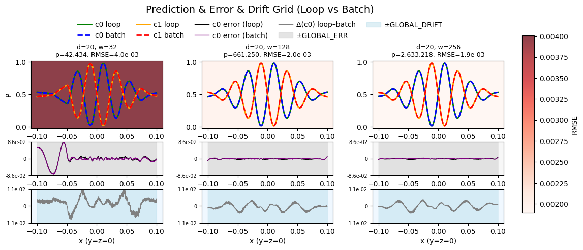
Figure 3a: Default (with TF32) kernel drift error.
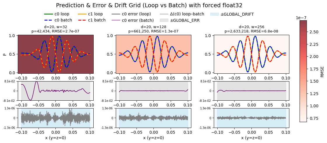
Figure 3b: FP32 kernel drift error.
Empirical observation
Across different widths, we measured (light blue background)
\[\Delta(x)\;=\;P_0^{\rm loop}(x)\;-\;P_0^{\rm batch}(x)\]and summarised each configuration by \(\mathrm{RMSE}(\Delta)\). we see (for the 4060ti 16GB):
- Drift starts small at very narrow widths.
- It peaks at intermediate widths (a few hundred).
- Then it falls off again at large widths, where both loop and batch paths happen to use the same kernel.
This non-monotonic pattern arises because XLA’s choice of GPU reduction kernels and their internal tiling depend on matrix dimensions. At certain sizes, the two pipelines diverge and coincide at others.
Remedies
- Uniform reductions: Force a single, full-precision FP32 path (no mixed-precision or fast-math shortcuts) so both modes use identical kernels. However, this still does not guarantee bitwise-identical results.
- Higher precision: Run critical inference in FP64 or a deterministic 64-bit-mantissa format, this also like the first remedy only pushes down the error further.
- Pad Batches: If we pad all our calls and use the same batch, we can atleast make the error reproducible.
Appendix
Bounds for error accumulation
First let’s get started with the smallest unit. Since most frameworks have the default setting of float32 we’ll assume that for now. For IEEE‑754 single‑precision arithmetic every real number \(z\) is rounded by
The relative error is bounded by \(u\); the absolute error scales with \(\lvert z\rvert\).
Now let’s extend this to the dot product. Let
\[z=\sum_{k=1}^n a_k b_k,\qquad \widehat z=\operatorname{fl}(z).\]Giving us:
\[\widehat z = z\,(1+\delta),\quad |\delta|\le\gamma_n,\quad \gamma_n := \frac{n\,u}{1 - n\,u}\approx n\,u. \tag{2}\]Proof for \(\gamma_n\)
By compounding the worst‐case rounding factor \((1+u)\) over \(n\) operations, the relative error satisfies \(|\delta_n|\le (1+u)^n - 1 \;\le\;\sum_{k=1}^n\binom{n}{k}u^k \;\le\;\sum_{k=1}^n(nu)^k \;=\;\frac{n\,u}{1 - n\,u} \;=\;\gamma_n.\)
Specifically:
- Binomial theorem: \((1+u)^n = \sum_{k=0}^n\binom{n}{k}u^k\;\Longrightarrow\;(1+u)^n - 1 = \sum_{k=1}^n\binom{n}{k}u^k\)
- Bound coefficients: \(\binom{n}{k}\le n^k\;\Longrightarrow\;\binom{n}{k}u^k\le(nu)^k\)
- Geometric‐series sum: \(\sum_{k=1}^n(nu)^k = (nu) + \cdots + (nu)^n\)
- Closed‐form: \(\displaystyle\sum_{k=1}^n(nu)^k = \frac{n\,u}{1 - n\,u} = \gamma_n\)
Intuition: \((1+u)^n - 1\) is the multiplicative snowball after \(n\) roundings
Error in the linear map
Let
\[y = W x \in \mathbb{R}^m,\qquad \hat y = \operatorname{fl}(Wx).\]By \((2)\) each length-\(n\) dot-product satisfies
\[\hat y_i = y_i\,(1+\delta_i),\quad |\delta_i|\le \gamma_n, \qquad \gamma_n := \frac{n\,u}{1 - n\,u}\approx n\,u.\]Hence for each neuron \(i\)
\[|\hat y_i - y_i|\le \gamma_n\,|y_i| \quad\Longrightarrow\quad \|\hat y - y\|_\infty \le \gamma_n\,\|y\|_\infty.\]Side note: \(\|\cdot\|_\infty\) simply picks out the worst‐case single‐neuron error, so we get one uniform bound across all \(m\) neurons.
Full layer with 1-Lipschitz activation
Define
\[y = W^{(\ell)}x^{(\ell)},\quad \hat y = \operatorname{fl}(y),\quad x^{(\ell+1)} = \sigma(y),\quad \hat x^{(\ell+1)} = \sigma(\hat y),\]where \(\sigma\) (ReLU, tanh, …) obeys
\[\|\sigma(v)-\sigma(w)\|_\infty \le \|v-w\|_\infty.\]Then
\[\|\hat x^{(\ell+1)} - x^{(\ell+1)}\|_\infty \;\le\;\|\hat y - y\|_\infty \;\le\;\gamma_{n_\ell}\,\|y\|_\infty \;\le\;\gamma_{n_\ell}\,\|x^{(\ell+1)}\|_\infty.\]So for each neuron \(i\) in layer \(\ell+1\)
\[|\hat x_i^{(\ell+1)} - x_i^{(\ell+1)}|\le \gamma_{n_\ell}\,|x_i^{(\ell+1)}|,\]and we write
\[\hat x^{(\ell+1)} = x^{(\ell+1)}\,(1+\delta^{(\ell)}),\quad |\delta^{(\ell)}|\le \gamma_{n_\ell}. \tag{3}\]Side note: \(\gamma_{n_\ell}\) uses the layer’s incoming dimensionality \(n_\ell\) (e.g. 256 inputs ⇒ \(\gamma_{256}\)) to bound every neuron’s relative slip.
How the next layer sums up errors.
The \(\infty\)-norm bound above compresses all per-neuron slips into one scalar \(\delta^{(\ell)}\). When these perturbed activations \(\hat y\) enter the next layer’s dot-product, \((2)\) on a length-\(n_{\ell}\) dot-product automatically sums whatever errors remain:
\[|\widehat z_j - z_j| \;=\;\Bigl|\sum_{i}w_{ji}\,\hat y_i - \sum_{i}w_{ji}\,y_i\Bigr| \;\le\;\gamma_{n_{\ell+1}}\sum_i|\hat y_i| \;\le\;\gamma_{n_{\ell+1}}\,n_{\ell+1}\,\|\hat y\|_\infty.\]Thus the “sum over all neurons” happens inside each subsequent dot-product bound, without ever unpacking the single \(\infty\)-norm scalar.
Accumulated Error Across \(L\) Layers
Chaining these per-layer relative slips gives
\[\hat f(x) = f(x)\prod_{\ell=0}^{L-1}(1+\delta^{(\ell)}) = f(x)\,\bigl(1+\varepsilon_{\rm acc}(x)\bigr),\]Direct‐expansion
\[\prod_{\ell=0}^{L-1}(1+\delta^{(\ell)})\]by distributing out each factor, you get one term for each single \(\delta^{(\ell)}\), plus terms involving products of two or more \(\delta\)s. Because each \(\delta^{(\ell)}=O(u)\), any product \(\delta^{(i)}\delta^{(j)}\) is \(O(u^2)\) and hence negligible at single precision. Dropping those higher-order terms leaves exactly
\[1 \;+\;\sum_{\ell=0}^{L-1}\delta^{(\ell)} + O(u^2).\]
where to first order and using \((3)\)
\[\varepsilon_{\rm acc}(x) = \sum_{\ell=0}^{L-1}\delta^{(\ell)} + O(u^2), \quad |\varepsilon_{\rm acc}|\le \sum_{\ell=0}^{L-1}\gamma_{n_\ell}.\]To reinforce: Each \(\gamma_{n_\ell}\) already folded in the sum of that layer’s neuron-level errors, so summing \(\gamma_{n_\ell}\) over \(\ell\) neatly captures the network’s total forward error.
Note on Conditioning
A more rigorous analysis replaces each \(\gamma_{n_\ell}\approx n_\ell\,u\) by a data-dependent bound \((\kappa_\ell,\,n_\ell,\,u)\), where the dot-product condition number \(\kappa_\ell \;=\; \frac{\sum_{k=1}^n |a_k b_k|}{\bigl|\sum_{k=1}^n a_k b_k\bigr|}\) captures any cancellation or scaling in that layer. Including \(\kappa_\ell\) refines the bound but does not alter its overall form.
Citation
Please cite this work as:
Or use the BibTeX citation:
@article{ vira2025neuralnetworkprecisionpitfallsinthewild,
  title="Neural Network precision pitfalls in the wild",
  author={Vira, Jash},
  journal={jashvira.github.io},
  year={2025},
  month={May},
  url={https://jashvira.github.io/blog/2025/nn_precision_pitfalls/}
}